Analytical Instrument Documents

From Uncertainty Report to Variance Analysis

Deviation in the Uncertainty Report:
The Uncertainty Report calculates Expanded Uncertainty by analyzing interactions between individual factors and overall data variations. This serves as a critical foundation for integrated analysis of uncertainty across the entire measurement process.

Role of Variance Analysis:
Variance analysis (ANOVA: Analysis of Variance) is a statistical method for determining how multiple factors in data affect the results. It isolates the pure deviations of each factor and clarifies their contribution levels. By separating interactions between factors, ANOVA establishes a solid basis for detailed analysis of uncertainty sources.

Comparison Through the ANOVA Report:
The results of the ANOVA Report allow for thorough analysis of uncertainty sources and the contribution rates of individual factors. This facilitates the development of clear guidelines for improving the measurement process. Such analysis plays an essential role in enhancing data reliability and accuracy.

Variance Analysis: Two-way ANOVA

Two-way ANOVA (Two-factor Analysis of Variance) is a method used to evaluate the effects of two different factors (Factor A and Factor B) on data, as well as their interaction. Below are the primary elements involved in the calculation:

1. Factor A Evaluates the impact of Factor A on the data.

2. Factor B Evaluates the impact of Factor B on the data.

3. Interaction Assesses the effects of the interaction between Factor A and Factor B on the data (Factor A × Factor B).

4. Error Represents random variability not attributable to the above factors or their interaction.

The Total Variance is determined by combining the contributions of all these elements (Factor A, Factor B, Interaction, and Error). Figure 1 illustrates the mechanism of Two-way ANOVA through a schematic diagram.

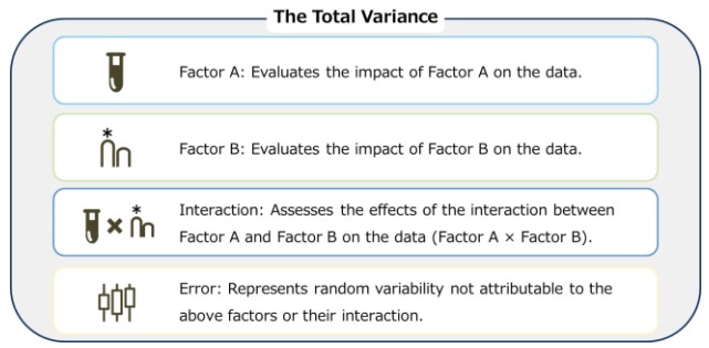
Figure 1. Schematic Diagram of Two-way ANOVA

JASON ANOVA: 2 way ANOVA

JASON Variance Analysis provides reports based on two distinct analytical models. The JASON 2 way ANOVA focuses on the effects of independent factors, offering a simple method for individually evaluating elements that influence the data. Its main features include:

• Factor A (Sample) Evaluates the independent contribution of Sample without considering direct relationships with Signal, treating it as a background element.

• Factor B (Signal) Assesses the direct impact of Signal on the data and evaluates its independent contribution.

• Interaction Does not include independent interaction terms.

This approach is particularly suitable when differences between samples are minimal or when the effects of Signal itself are the main focus. Compared to JASON’s other model, the 2-way nested ANOVA, it offers a simpler structure that is effective for analyzing individual factors. Figure 2 presents a schematic diagram illustrating the mechanism of the JASON 2 way ANOVA.

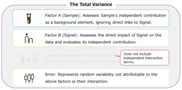
Figure 2. Schematic Diagram of JASON 2 way ANOVA

JASON ANOVA: 2-way nested ANOVA

JASON 2-way nested ANOVA is a comprehensive method for evaluating the relationships and interactions between multiple factors. Its main features include:

• Factor A (Sample) Assesses elements influencing data across multiple levels. Similar to the 2 way ANOVA, it is treated as a background factor.

• Factor B (Signal) Analyzes the direct impact on data, evaluating it in relation to the levels of Sample.

• Interaction Independent interaction terms are not included.

This model is particularly suitable for scenarios where Sample's contribution is critical or where Signal's effect needs to be analyzed in conjunction with Sample interactions. It supports complex data analysis and yields more accurate results. Figure 3 illustrates a schematic diagram of the mechanism of JASON 2-way nested ANOVA. Additionally, Table 1 compares the differences between the two analytical models.

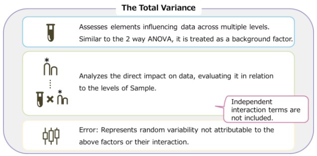
Figure 3. Schematic Diagram of JASON 2-way nested ANOVA

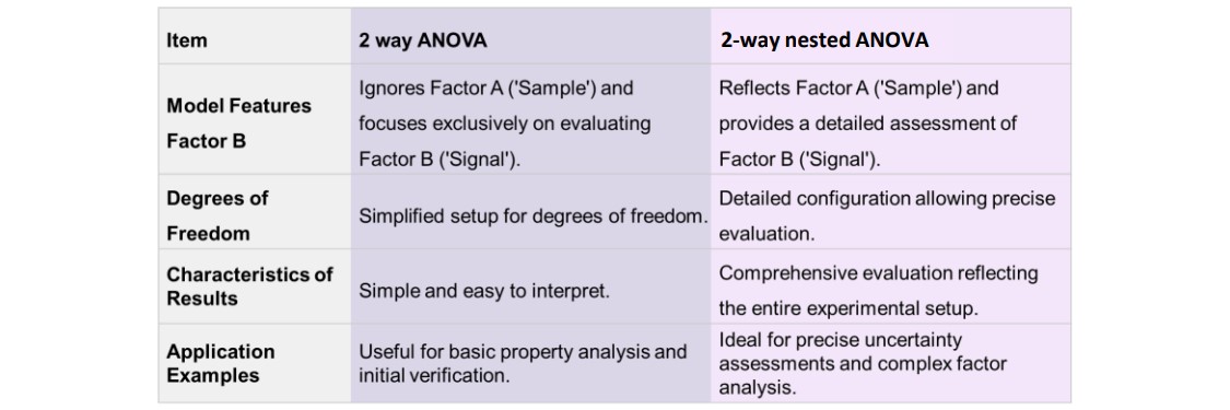
Table 1. Differences Between 2 way ANOVA and 2-way nested ANOVA

Details of the ANOVA Report

In the ANOVA report, variations attributed to each factor are calculated as Mean Square Variance, a key metric for interpreting variance analysis and quantitatively assessing the contribution of each factor. From the Mean Square Variance, deviations for individual factors can be calculated. These deviations, determined independently of other factors or interactions, are referred to as Pure Deviation. By using Pure Deviation, it is possible to extract uncertainty that captures the impact of each factor individually. This process quantitatively evaluates the precision and reliability of the data, laying the groundwork for deeper insights into analytical results. Figure 4 provides an overview of the metrics included in the 2 way ANOVA report, along with detailed explanations.

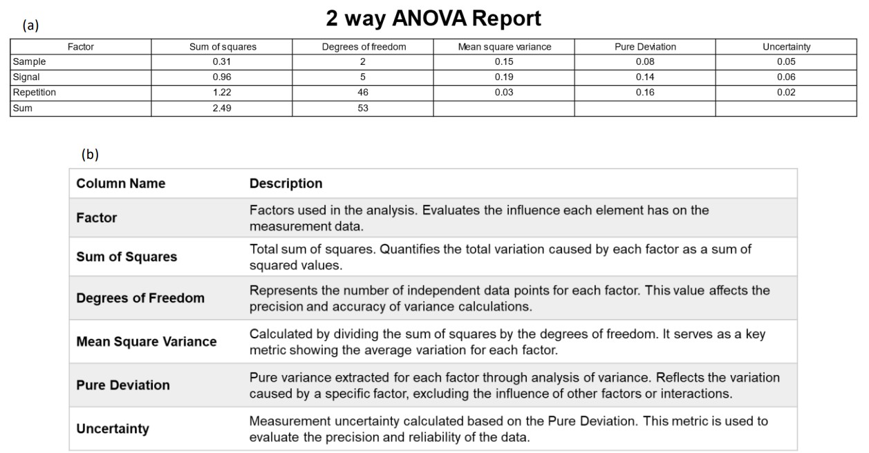
Figure 4. ANOVA Report: (a) 2 way ANOVA report, (b) Metrics and Descriptions

Comparison Between 2 way ANOVA and Uncertainty Report Results

Figure 5 compares the results of the 2 way ANOVA and the uncertainty report (Application Note NM250002) using a radar chart. The purple color represents the results of the 2 way ANOVA, while the blue color indicates the results of the uncertainty report. The following trends are observed:

• Sample Shows lower values compared to the uncertainty report, suggesting that only the pure effects have been extracted.

• Signal Displays smaller values, clearly indicating that the influence of other factors and interactions has been reduced.

• Repetition Shows very small values, reflecting a high level of stability in the measurement process itself.

Differences between the Results of the Uncertainty Report The differences between the results of the two reports can be explained by the characteristics outlined in Table 2. The uncertainty report provides an evaluation that considers the "worst-case scenario" and tends to assess repeated errors as relatively large. On the other hand, variance analysis offers an approach that reflects the "overall characteristics of the data," extracting uncertainties isolated from other factors. Additionally, variance analysis enables detailed analysis of individual factors.

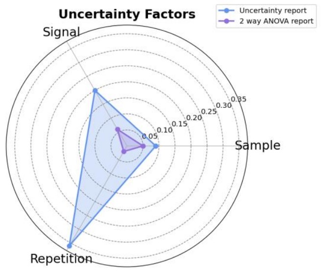
Figure 5. Comparison Between 2 way ANOVA and Uncertainty Report Results

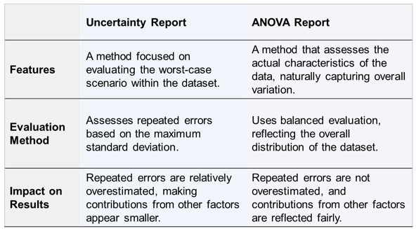
Table 2. Key Characteristics of the Uncertainty and ANOVA  Reports

Analysis of Differences from the Uncertainty Report Results

To analyze the differences from the uncertainty report results, the following steps are undertaken to examine the variance analysis outcomes. First, the validity of the variance analysis results is verified. Then, an analysis of factors is conducted using the results of the two variance analysis models.

1. Verification of Data Statistical Properties
   The statistical properties of the underlying data are evaluated to confirm the validity of the uncertainty and variance analysis results. The report data was analyzed using Python for this evaluation. The following methods were employed:
   • IQR Test
   • Shapiro-Wilk Test
   • QQ Plot
   • KDE Plot
2. Factor Assessment in Variance Analysis
   The contribution of data variability and uncertainty to each factor is assessed. This process involves comparing the results of the 2 way ANOVA and the 2-way nested ANOVA to organize the relative impact of each factor.

1. Verification of Data Statistical Properties: Outlier Examination (IQR Test)

The IQR Test (Interquartile Range Method) is one of the techniques used to detect outliers in data. The IQR is defined as the difference between the third quartile (Q3) and the first quartile (Q1), representing the range of the central 50% of the data. In the box plot shown in Figure 6, the following elements are illustrated:

• Box (IQR): Represents the range from Q1 to Q3.
• Line inside the Box: Indicates the median of the data (50th percentile).
• Whiskers: Represent the overall range of the data.

As a result of this analysis, no outliers were detected, and it was confirmed that the variability within the data is small.

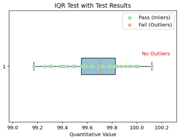
Figure 6. IQR Test Results

1. Verification of Data Statistical Properties: Normality Check

Shapiro-Wilk: Test The Shapiro-Wilk test is a statistical method for testing the normality of data. In this test, the null hypothesis assumes that "the data follows a normal distribution." The calculated p-value of 0.6092 is significantly greater than 0.05, confirming that the data follows a normal distribution.

QQ Plot (Quantile-Quantile Plot): The QQ plot is used to compare the distribution of data against a theoretical normal distribution. The closer the points of the actual data align with the straight line representing the theoretical values, the higher the normality. Figure 7 (a) illustrates the QQ plot created using the calculated results. This plot statistically confirms the normality of the data.

KDE Plot (Kernel Density Estimate): The KDE plot is a method for smoothing the distribution of data, providing a more accurate display of data density compared to histograms. Figure 7 (b) shows the KDE plot created using the calculated results. This plot visually confirms the normality of the data.

Assessment of Variance Analysis Validity: Based on the verification results from the above methods, the validity of the variance analysis has been confirmed. Normality has been evaluated both statistically and visually, providing a reliable foundation for trustworthy analytical results.

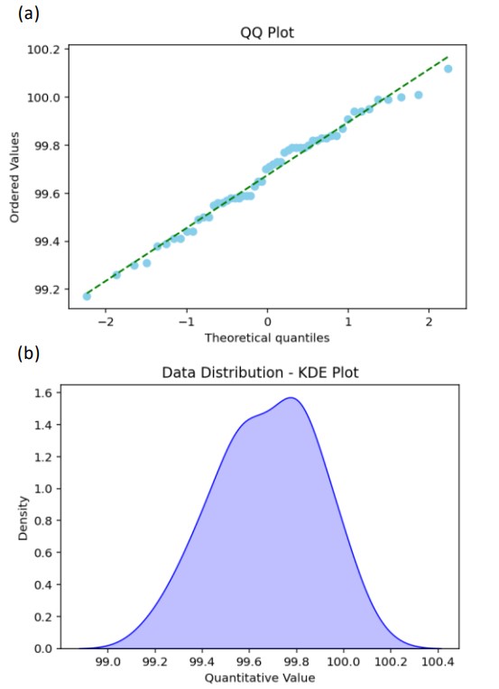
Figure 7. Verification of Data Statistical Properties: (a) QQ Plot, (b) KDE Plot

2. Factor Assessment in Variance Analysis

Figure 8 compares the results of the 2 way ANOVA and 2-way nested ANOVA using a radar chart. The purple color represents the results of the 2 way ANOVA, while the darker purple indicates the results of the 2-way nested ANOVA. The following trends were observed:

• Sample Both models show similar values, confirming the stability of variability. However, the 2 way ANOVA results suggest the potential influence of interactions with other factors.

• Signal The 2-way nested ANOVA shows lower values, while the 2 way ANOVA produces relatively higher values. These findings indicate that the Signal might be sensitive to repeated errors, Sample, or interactions with standard samples.

• Repetition The values for repeated errors are nearly identical across both models (0.02), confirming a high degree of stability. Additionally, it was noted that the overall variability of the measurement data is kept to a minimum.

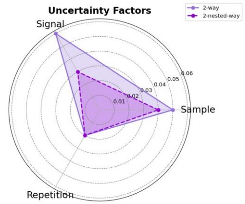
Figure 8. Results of JASON ANOVA

Summary of Variance Analysis Results

Based on comparisons with the uncertainty report, the following points have been confirmed through variance analysis:

• Validity of Variance Analysis The uncertainty associated with each factor has been statistically validated, and its influence on quantitative analysis results has been clarified.

• Repeated Errors Repeated errors show extremely small values, supporting the stability of the measurement process and reliability of the data.

• Impact of Standard Samples The uncertainty from standard samples has been found to propagate throughout the measurement, establishing them as key influential factors.

• Impact of Interactions Interactions between Signal and Sample may contribute to the uncertainty within the measurement data.

These findings provide critical insights for enhancing the reliability of quantitative analysis.

How Does the Uncertainty of Standard Samples Impact Quantitative Analysis Results?

From the previous analysis, it has been confirmed that repeated errors across the entire measurement system are very small, demonstrating the stability of the measurement process. However, further investigation is needed to explore how the uncertainty associated with standard samples affects the measurement results. To address this issue, detailed analyses using methods such as simulations would be effective. Particularly, evaluating the impact of standard sample characteristics on the overall data can provide crucial insights to improve measurement accuracy and reliability. The detailed exploration of this analysis will be covered in "Part 3. Elucidating Factors through Simulation Analysis."

---

[1] JEOL Analytical Software Network
[2] Spectral Management Interface Launching Engine for Q-NMR

Attached Files

• QNMR analysis improving accuracy part 2 nm250003_2.pdf 763 KB